Comp578 Susan Portugal Fall 2008
Assignment 11 November 13, 2008
10.7.1
Compare and contrast the different techniques for anomaly detection that were presented in Section 10.1.2. In particular, try to identify circumstances in which the definitions of anomalies used in the different techniques might be equivalent or situations in which one might make sense, but another would not. Ensure you consider different types of data.
There are three different anomaly detection techniques described in section 10.1.2: Model-Based Techniques, Proximity-Based Techniques, and Density-Based Techniques. Model-Based Techniques create a model of the data and identifies objects that do not fit the model. Although, when the data cannot be modeled for the statistical distribution of the data, the following two Techniques can be used. Proximity-Based Techniques measure the distance from most of the other objects and classifies the distant objects as anomalies. Density-Based Techniques estimate the density of the data and areas of low density are considered an anomaly. Density-Based and Proximity-Base Techniques are similar in how they analyze the distance between objects. Both of these Techniques can also be expressed as a Model-Based Techniques depending upon the established constraints of the data set.
10.7.8.
Many statistical tests for outliers were developed in an environment in which a few hundred observations was a large data set. We explore the limitations of such approaches.
a. For a set of 1,000,000 values, how likely are we to have outliers according to the test that says a value is an outlier if it is more than three standard deviations from the average? (Assume a normal distribution.)
To perform an analysis on the given situation, a Gaussian distribution can be applied. The two pieces of information need is the distribution (0.0027) probability that a data point/object outside of the central area of plus or minus 3 standard deviations as the second piece of information. The following can be performed to find the number of outliers:
0.0027 x 1,00,00 = 2700 total outliers
b. Does the approach that states an outlier is an object of unusually low probability need to be adjusted when dealing with large data sets? If so, how?
When dealing with large data set the analysis can have a different approach in classifying outliers. Outlier is defined by its distance from the central object data set in comparison to other objects in the data set. Depending on the precision of the data set and outlier can be at future distance from the central of the data set greater than a defined radial distance.
10.7.9.
The probability density of a point x with respect to a multivariate normal distribution having a mean μ and covariance matrix Σ is given by the equation
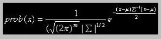
Using the sample mean x and covariance S as estimates of the mean μ and covariance matrix Σ respectively, show that the log prob(x) is equal to the Mahalanobis distance between a data point x and the sample mean x plus a constant that does not depend on x.
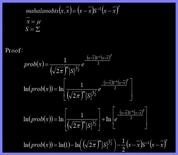
With the proof above, log prob(x) is equal to the Mahalanobis distance between a data point x and the sample mean x plus a constant that does not depend on x.
