Comp578 Susan Portugal Fall 2008
Project December 4, 2008
Reflectance Round Robin Data Mining Analysis
The following final Data Mining Project includes data that was collected for a standards committee for the fiber optic industry. Below there is a description of the data that was collected, along with a data mining analysis of the data; including scatter plots, mean, range, variance, and anomaly detection within the data set. Once the analysis is complete, the end results will demonstrate the limits within the Reflectance measurement.
The evolvement of a complex unit into a workable “standard” often involves the cooperation of innovative minds. For the singlemode fiber optic connectors, several members within the fiber optic industry agreed to participate in testing several fiber optic connectors in order to determine and/or develop the repeatability and reliability (R&R) of the reflectance of a fiber optic connector. This “round robin” of participants were give an instruction list of specific steps in testing the connector samples in order to determine the deviant of reflector sample.
The sample being tested involves an FC-APC ( a standardized fiber optic connector with an angle polished ceramic ferrule). A standard FC connector consists of a threaded key-locking mechanism for single directional mounting. The APC consists of an eight to nine degree angled ferrule with a radius of a curvature between five and 12 mm. The APC connector has become the connector of choice by the fiber optic market due to its diminished level of reflective distortion.
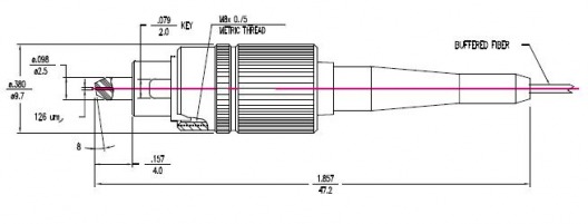
(Figure 1--FC Style Connector Diagram)
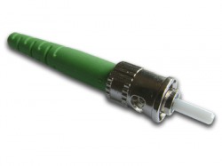
(Figure 2--FC Style Connector Actual Picture)
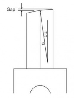
(Figure 3--APC Ferrule Diagram (8-9 Degree Angled Tip))
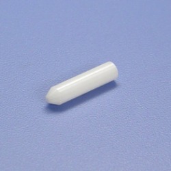
(Figure 4--APC Ferrule Picture (8-9 Degree Angled Tip)
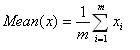
Reflectance loss and/or return loss is a ratio of the amount of power reflected relative to the transmitted signal power source in decibels (dB). in this whether the results specified achieving the desired measurement of with known reflectance.
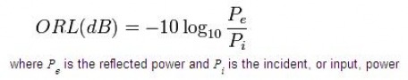
(Figure 5--Reflectance/Return Loss Equation)
With the use of several different Data Mining Methods learned throughout course the following analysis can be performed to depict the variance and standardization of the Reflectance Measurement.
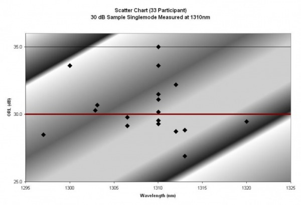
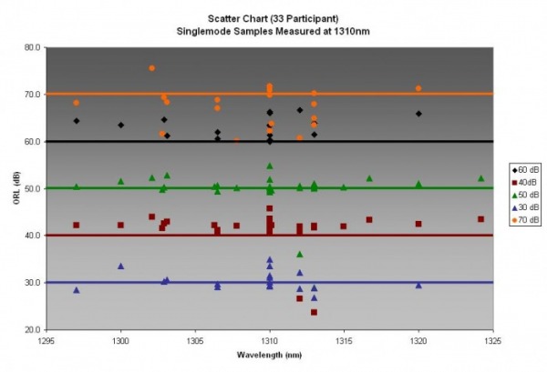
Scatter Plots
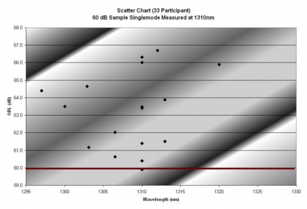
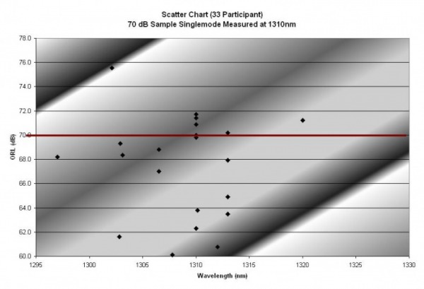
Scatter Plots overall depicts the data set for the five sample groups: 30 dB, 40 dB, 50 dB, 60 dB, and 70 dB. Each scatter chart varies by the exact wavelength and the corresponding ORL measurement.
Mean Analysis
Mean(30dB) = 30.5 dB Delta = 0.5 dB
Mean(40dB) = 41.1 dB Delta = 1.1 dB
Mean(50dB) = 49.7 dB Delta = 0.3 dB
Mean(60dB) = 63.3 dB Delta = 3.3 dB
Mean(70dB) = 67.5 dB Delta = 2.5 dB
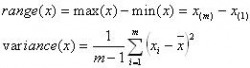
Range Analysis and Variance Analysis revealing the spread between the data set. Variance can be a more accurate analysis when there are extreme values within the data set.
Range(30dB) = 8.1 dB Variance(30dB)= 4.03 dB
Range(40dB) = 22.1 dB Variance(40dB) = 18.80 dB
Range(50dB) = 25.9 dB Variance(50dB) = 21.51 dB
Range(60dB) = 6.8 dB Variance(60dB) = 4.61 dB
Range(70dB) = 15.4 dB Variance(70dB) = 16.51 dB
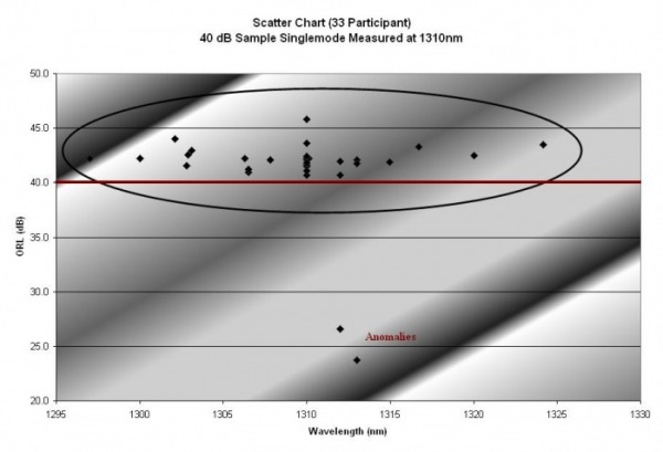
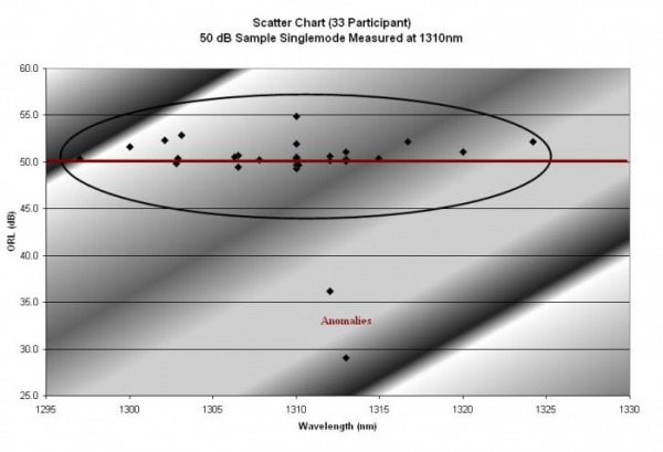
Anomaly Detection
There are three different anomaly detection techniques described in Introduction to Data Mining by Pang-Ning Tan in section 10.1.2: Model-Based Techniques, Proximity-Based Techniques, and Density-Based Techniques. Model-Based Techniques create a model of the data and identifies objects that do not fit the model. Although, when the data cannot be modeled for the statistical distribution of the data, the following two Techniques can be used. Proximity-Based Techniques measure the distance from most of the other objects and classifies the distant objects as anomalies. Density-Based Techniques estimate the density of the data and areas of low density are considered an anomaly. Density-Based and Proximity-Base Techniques are similar in how they analyze the distance between objects. Both of these Techniques can also be expressed as a Model-Based Techniques depending upon the established constraints of the data set.
Using the model anomly dection method building a model of around the nominal value of the given sample and a threshold of data points greater than or less than 10 dB. From this analysis, two data sets have anomalys, 40 dB and 50 dB.
After the anomalies are located within the data sets of 40 dB and 50 dB the following comparison between the mean, the difference between the mean and the nomial value, range and bariance can be performed. Overall the difference between the mean and the nomial value increased while the range, spread, decrease significantly.
Mean(30dB) = 30.5 dB Delta = 0.5 dB
Mean(40dB) = 41.1 dB→42.2 dB Delta = 1.1 dB→2.2 dB
Mean(50dB) = 49.7 dB→50.8 dB Delta = 0.3 dB→0.8dB
Mean(60dB) = 63.3 dB Delta = 3.3 dB
Mean(70dB) = 67.5 dB Delta = 2.5 dB
Range(30dB) = 8.1 dB Variance(30dB)= 4.03 dB
Range(40dB) = 22.1 dB→5.1 dB Variance(40dB) = 18.80 dB→1.10 dB
Range(50dB) = 25.9 dB→5.6dB Variance(50dB) = 21.51 dB→1.35 dB
Range(60dB) = 6.8 dB Variance(60dB) = 4.61 dB
Range(70dB) = 15.4 dB Variance(70dB) = 16.51 dB
